Deep learning(CNN)

说在前面的话：长文预警。除了介绍CNN外，还有许多作者对当前深度学习及AI行业的见解。另外，配置theano真的恶心（无奈代码用的是theano，否则早用tensorflow了，我的anaconda是卸了装，装了卸，到现在还没搞好），所以目前代码都没跑过，只能阅读分析了。

在介绍CNN前，先看一下network3.py中的FullyConnectedLayer类：

class FullyConnectedLayer(object):
    
    def __init__(self, n_in, n_out, activation_fn=sigmoid, p_dropout=0.0):
        self.n_in = n_in
        self.n_out = n_out
        self.activation_fn = activation_fn
        self.p_dropout = p_dropout
        # Initialize weights and biases
        self.w = theano.shared(
            np.asarray(
                np.random.normal(
                    loc=0.0, scale=np.sqrt(1.0/n_out), size=(n_in, n_out)),
                dtype=theano.config.floatX),
            name='w', borrow=True)
        self.b = theano.shared(
            np.asarray(np.random.normal(loc=0.0, scale=1.0, size=(n_out,)),
                       dtype=theano.config.floatX),
            name='b', borrow=True)
        self.params = [self.w, self.b]

    def set_inpt(self, inpt, inpt_dropout, mini_batch_size):
        self.inpt = inpt.reshape((mini_batch_size, self.n_in))
        self.output = self.activation_fn(
            (1-self.p_dropout)*T.dot(self.inpt, self.w) + self.b)
        self.y_out = T.argmax(self.output, axis=1)
        self.inpt_dropout = dropout_layer(
            inpt_dropout.reshape((mini_batch_size, self.n_in)), self.p_dropout)
        self.output_dropout = self.activation_fn(
            T.dot(self.inpt_dropout, self.w) + self.b)

    def accuracy(self, y):
        "Return the accuracy for the mini-batch."
        return T.mean(T.eq(y, self.y_out))

init就是初始化一些参数，这里bias初始化为(n_out,)形状，其实就是一个n_out列的一维数组，这样使得它在后续的运算中有扩展性，可以同时加到mini_batch个数据上。需要注意p_dropout是被dropout的概率，因为我们要使用dropout方法了（具体实施后面会说），初始化权重和bias时采用的是theano的共享变量，指出了变量名分别为’w’和’b’，borrow参数设置为True，表示变量可以被后续操作更改。set_inpt方法是输入数据并计算出output的，注意设置input时用了两种方法，self.inpt和self.output用于validation和test，它们没用用dropout，虽然输出时前面乘了(1-self.dropout)，但这只是把所有元素都缩放了相同的倍数，实际上并没有用到dropout（虽然我不知道到底乘了干嘛）。self.inpt_dropout和self.output_dropout用于train，它们真正用了dropout，其中的dropout_layer函数如下：

def dropout_layer(layer, p_dropout):
    srng = shared_randomstreams.RandomStreams(
        np.random.RandomState(0).randint(999999))
    mask = srng.binomial(n=1, p=1-p_dropout, size=layer.shape)
    return layer*T.cast(mask, theano.config.floatX)

由于不了解theano，我只能知道它的大体思想是通过随机流srng生成一个与layer同shape的二项分布，将其数据格式转换成与w、b相同的theano.config.floatX后与layer做内积，这样就达到了随机舍弃部分neuron的目的，注意舍弃的数目由p_dropout控制。这个函数我觉得很巧妙：将理论上的舍弃——即要么是0要么是1用二项分布实现。

Convolutional networks

之前的全连接网络总给人一种“暴力求解”的感觉，因为由于其全连接性，导致每一层似乎都把输入图像的许多特征都糅合起来，即没有考虑图像的空间结构spatial structure（说的有点模糊，意会即可），而CNN则很好地使用了图像的spatial structure。

Local receptive fields

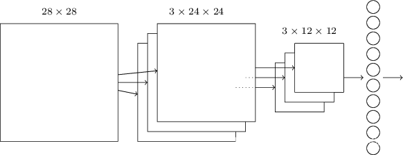
之前我们的输入是784×1的数据，现在CNN中的输入是28×28的数据，此时取一个固定大小的“窗口”，从图片左上角以一定的步长从左到右、从上到下移动到右下角，即（可能有重叠地）覆盖整张图片，每次移动，整个这个“窗口“的内容都会被映射成一个数字（具体方法接下来介绍）。这个”窗口“即为local receptive fields，移动的”步长“即为stride length，以5×5的”窗口“，步长1为例如下图：

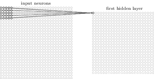
很容易看出原本28×28的图片经过这样的处理变成了24×24。

Shared weights and biases

和FC net相邻两层的神经元两两之间都有各自的weight不同，CNN采用共享的权重和偏置。
上面提到了以窗口为单位映射的方法，如何把一个窗口内数据映射为单个数值？仍以上面5×5的窗口为例，将其与一个5×5的weight做内积（即convolution，这也是CNN名字的由来）即可。事实上，对于窗口覆盖完图片这一整个过程，每次映射采用的weight都是一样的，至于bias则是在所有内积做完后再加上。于是这样一个不变的weight就可以想象提炼成图片的一个特征，随着窗口内数据的变化，得到的output内容也不同，并且其仍会呈现spatial structure。所以，这样一整个映射就是一次feature map，其weight和bias即为shared weight和shared bias，这两个参数也定义了kernel or filter(也就是原来的神经元，只不过由于共享参数它便具有了”过滤”特征的功能)。

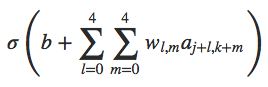
上式w是一个5×5的矩阵，显然(j,k)对应的是当前窗口左上角的”坐标“。

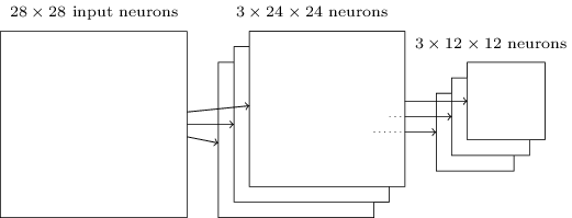
事实上，提取的特征也并不局限在一个，图像识别需要更多的特征——多搞几个weight就是了，早期的LeNet-5就采用了6个特征，其local receptive field也是5×5，所以，原本的28×28数据就变成了6×24×24的数据，也可以看成此时有了六个filter。将特征（20个）可视化可以更清楚地理解feature map的过程：

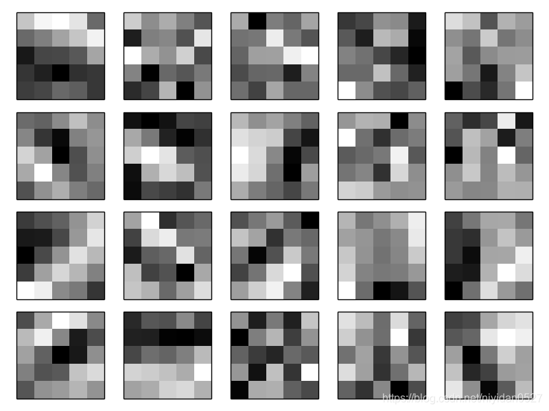
颜色较深的像素对应着较大的weight元素，反之则较小。其实最后训练好的weight有些可以看出其对应feature，比如轮廓等，但大部分是看不懂的。
于是，CNN参数显然远远少于FC net，这就意味着更高的学习速度，更深的网络。这里再贴出我的一张笔记：

Pooling layers

池化层通常紧跟着卷积层，作用是简化信息——其实就类似于缩小图片。max-pooling是很常用的一种池化方法，在卷积层的24×24取一个窗口（先以一个feature为例），不妨设窗口大小为2×2，取其中灰度值最大的像素（如果是RGB三色通道貌似看RGB平均值），其他三个像素丢弃，如下图（貌似池化层的窗口不重叠）：

实际操作效果就类似于缩小图片。这里了解一个概念：平移不变性，我只是偶然想到这个概念，[知乎这个回答](深度学习cnn中，怎么理解图像进行池化（pooling）后的平移不变性？ - 三符的回答 - 知乎 https://www.zhihu.com/question/34898241/answer/60705313)感觉说的不错，这位答主还提到了***average pooling（另一种池化方法，此外还有L2 pooling***——取窗口数据的均方根）对背景保留更好，max pooling对纹理提取更好。可见相对于其他特征，某个特征的具体位置并不算重要。
对于多个feature map，每一个map后的output都要pooling：

需要说明的是，这里把pooling layer单独看作一层，但由于其往往连在卷积层之后，所以它和卷积层也可以一起看作一层，即convolutional-pooling layers：

class ConvPoolLayer(object):

    def __init__(self, filter_shape, image_shape, poolsize=(2, 2),
                 activation_fn=sigmoid):
        """`filter_shape` is a tuple of length 4, whose entries are the number
        of filters, the number of input feature maps, the filter height, and the
        filter width.

        `image_shape` is a tuple of length 4, whose entries are the
        mini-batch size, the number of input feature maps, the image
        height, and the image width.

        `poolsize` is a tuple of length 2, whose entries are the y and
        x pooling sizes.

        """
        self.filter_shape = filter_shape
        self.image_shape = image_shape
        self.poolsize = poolsize
        self.activation_fn=activation_fn
        # initialize weights and biases
        n_out = (filter_shape[0]*np.prod(filter_shape[2:])/np.prod(poolsize))
        self.w = theano.shared(
            np.asarray(
                np.random.normal(loc=0, scale=np.sqrt(1.0/n_out), size=filter_shape),
                dtype=theano.config.floatX),
            borrow=True)
        self.b = theano.shared(
            np.asarray(
                np.random.normal(loc=0, scale=1.0, size=(filter_shape[0],)),
                dtype=theano.config.floatX),
            borrow=True)
        self.params = [self.w, self.b]

    def set_inpt(self, inpt, inpt_dropout, mini_batch_size):
        self.inpt = inpt.reshape(self.image_shape)
        conv_out = conv.conv2d(
            input=self.inpt, filters=self.w, filter_shape=self.filter_shape,
            image_shape=self.image_shape)
        pooled_out = pool_2d(
            input=conv_out, ws=self.poolsize, ignore_border=True)
        self.output = self.activation_fn(
            pooled_out + self.b.dimshuffle('x', 0, 'x', 'x'))
        self.output_dropout = self.output # no dropout in the convolutional layers

有一点疑惑是，在初始化权重时，根据注释，假设filter_shape=(20,1,5,5)，那么n_out就等于20×(5×5)/(2×2)=125，有点搞不明白。倒数第二行的dimshuffle()方法可以把原本shape为(20,)的bias转换为(1,20,1,1)shape，由此可见输出的shape为(1,20,1,1)，但theano中conv_2d、pool_2d方法具体运算过程我还是没有透彻了解，这里需要加强学习。

Putting it all together

至于最后的输出，只要在最后加一个FC层即可：

FC层的十个neuron与池化层的三个neuron（应该是3个吧）全连接，训练方法与FC net一样采用SGD和BP算法，只不过其具体过程不似之前那般简单，作者也以Problem的形式提出来，我暂且还没有思考。
上面是最简单的CNN，其实卷积池化层、FC层的数量都不限于一个，择优录取即可。

FC层默认的激励函数是sigmoid，然而输出层还可以用Softmax（更常见）:

class SoftmaxLayer(object):

    def __init__(self, n_in, n_out, p_dropout=0.0):
        self.n_in = n_in
        self.n_out = n_out
        self.p_dropout = p_dropout
        # Initialize weights and biases
        self.w = theano.shared(
            np.zeros((n_in, n_out), dtype=theano.config.floatX),
            name='w', borrow=True)
        self.b = theano.shared(
            np.zeros((n_out,), dtype=theano.config.floatX),
            name='b', borrow=True)
        self.params = [self.w, self.b]

    def set_inpt(self, inpt, inpt_dropout, mini_batch_size):
        self.inpt = inpt.reshape((mini_batch_size, self.n_in))
        self.output = softmax((1-self.p_dropout)*T.dot(self.inpt, self.w) + self.b)
        self.y_out = T.argmax(self.output, axis=1)
        self.inpt_dropout = dropout_layer(
            inpt_dropout.reshape((mini_batch_size, self.n_in)), self.p_dropout)
        self.output_dropout = softmax(T.dot(self.inpt_dropout, self.w) + self.b)

    def cost(self, net):
        "Return the log-likelihood cost."
        return -T.mean(T.log(self.output_dropout)[T.arange(net.y.shape[0]), net.y])

    def accuracy(self, y):
        "Return the accuracy for the mini-batch."
        return T.mean(T.eq(y, self.y_out))

与之前的layer大体相同，一点不同是，Softmax将权重和偏置都初始化为0，因为之前对它们初始化的方法的讨论都是基于sigmoid的，对Softmax未必适用，所以干脆直接初始化为0。另外里面还用到了theano的softmax网络，具体还要去看theano手册。
有了基本的layer，就可以用他们搭建一个网络了，初始化过程包括各种参数以及前向计算方法：

class Network(object):

    def __init__(self, layers, mini_batch_size):
        """Takes a list of `layers`, describing the network architecture, and
        a value for the `mini_batch_size` to be used during training
        by stochastic gradient descent.
        """
        self.layers = layers
        self.mini_batch_size = mini_batch_size
        self.params = [param for layer in self.layers for param in layer.params]#all weights and bias
        self.x = T.matrix("x")#a 2-d array whose name is "x"
        self.y = T.ivector("y")#a vector whose elements are int
        init_layer = self.layers[0]
        init_layer.set_inpt(self.x, self.x, self.mini_batch_size)
        for j in range(1, len(self.layers)):
            prev_layer, layer  = self.layers[j-1], self.layers[j]
            layer.set_inpt(
                prev_layer.output, prev_layer.output_dropout, self.mini_batch_size)
        self.output = self.layers[-1].output
        self.output_dropout = self.layers[-1].output_dropout

然后和之前的代码一样用SGD训练，先看一部分代码：

def SGD(self, training_data, epochs, mini_batch_size, eta,
        validation_data, test_data, lmbda=0.0):
    """Train the network using mini-batch stochastic gradient descent."""
    training_x, training_y = training_data
    validation_x, validation_y = validation_data
    test_x, test_y = test_data

    # compute number of minibatches for training, validation and testing
    num_training_batches = int(size(training_data)/mini_batch_size)
    num_validation_batches = int(size(validation_data)/mini_batch_size)
    num_test_batches = int(size(test_data)/mini_batch_size)

    # define the (regularized) cost function, symbolic gradients, and updates
    l2_norm_squared = sum([(layer.w**2).sum() for layer in self.layers])
    cost = self.layers[-1].cost(self)+\
           0.5*lmbda*l2_norm_squared/num_training_batches
    grads = T.grad(cost, self.params)
    updates = [(param, param-eta*grad)
               for param, grad in zip(self.params, grads)]

这里初始化了数据集，计算了三个数据集中各自mini_batch的数目，并且使用了L2 regularization，给出了cost的表达式和更新参数的公式，这里theano.tensor中的grad方法直接给出了cost对于weight和bias的导函数，大大减少了代码量。

# define functions to train a mini-batch, and to compute the
   # accuracy in validation and test mini-batches.
   i = T.lscalar() # mini-batch index(long int)
   train_mb = theano.function(
       [i], cost, updates=updates,
       givens={
           self.x:
           training_x[i*self.mini_batch_size: (i+1)*self.mini_batch_size],
           self.y:
           training_y[i*self.mini_batch_size: (i+1)*self.mini_batch_size]
       })
   validate_mb_accuracy = theano.function(
       [i], self.layers[-1].accuracy(self.y),
       givens={
           self.x:
           validation_x[i*self.mini_batch_size: (i+1)*self.mini_batch_size],
           self.y:
           validation_y[i*self.mini_batch_size: (i+1)*self.mini_batch_size]
       })
   test_mb_accuracy = theano.function(
       [i], self.layers[-1].accuracy(self.y),
       givens={
           self.x:
           test_x[i*self.mini_batch_size: (i+1)*self.mini_batch_size],
           self.y:
           test_y[i*self.mini_batch_size: (i+1)*self.mini_batch_size]
       })
   self.test_mb_predictions = theano.function(
       [i], self.layers[-1].y_out,
       givens={
           self.x:
           test_x[i*self.mini_batch_size: (i+1)*self.mini_batch_size]
       })

这段代码初看有点令人头大，但实际上非常简单，首先用T.lscalar()初始化一个long int用于表示mini_batch index，接下来的theano.function是重头戏，这里是该方法源码，这篇blog介绍的也很好，简单来说，该方法就是通过input（即第一个参数[i]）返回待计算的output（第二个参数，cost、accuracy等），计算过程中需要用到updates（如果有需要更新的参数，输入形式是(shared variables,update expression)）和givens（上面的代码用的是字典，每次都会根据input更新，但字典的key不变）。
所以，上面其实就是定义了四个函数，分别是训练cost、验证accuracy、测试accuracy和预测函数，前三个有点类似于network2.py中的四个指标。

接下来的代码用到了上面的四个函数：

# Do the actual training
        best_validation_accuracy = 0.0
        for epoch in range(epochs):
            for minibatch_index in range(num_training_batches):
                iteration = num_training_batches*epoch+minibatch_index
                if iteration % 1000 == 0:
                    print("Training mini-batch number {0}".format(iteration))
                cost_ij = train_mb(minibatch_index)
                if (iteration+1) % num_training_batches == 0:
                    validation_accuracy = np.mean(
                        [validate_mb_accuracy(j) for j in range(num_validation_batches)])
                    print("Epoch {0}: validation accuracy {1:.2%}".format(
                        epoch, validation_accuracy))
                    if validation_accuracy >= best_validation_accuracy:
                        print("This is the best validation accuracy to date.")
                        best_validation_accuracy = validation_accuracy
                        best_iteration = iteration
                        if test_data:
                            test_accuracy = np.mean(
                                [test_mb_accuracy(j) for j in range(num_test_batches)])
                            print('The corresponding test accuracy is {0:.2%}'.format(
                                test_accuracy))
        print("Finished training network.")
        print("Best validation accuracy of {0:.2%} obtained at iteration {1}".format(
            best_validation_accuracy, best_iteration))
        print("Corresponding test accuracy of {0:.2%}".format(test_accuracy))

iteration是迭代mini_batch的轮数，每满1000轮输出一条信息。一个epoch将所有的traning_batches迭代一遍，并且在每个epoch最后一次迭代后（cost_ij算完后）计算验证集accuracy，更新最佳验证精度，并记住最佳验证精度对应的迭代轮数best_iteration。

Practical application of CNN

为提高减少overfitting，作者通过expand_mnist.py手动扩大数据集，具体代码没有看，据作者自己介绍，是通过上下左右各移动一个pixel实现的，所以原来的50000条data就扩大到了250000条。另外，通过采用多FC层、将每个FC层neuron数增至1000、在其中使用dropout、用ReLU作为激励函数、采用Softmax等方法，最终作者得到了99.60％的准确率。

net = Network([
	ConvPoolLayer(image_shape=(mini_batch_size, 1, 28, 28),
				  filter_shape=(20, 1, 5, 5),
				  poolsize=(2, 2),
				  activation_fn=ReLU),
   ConvPoolLayer(image_shape=(mini_batch_size, 20, 12, 12),
				  filter_shape=(40, 20, 5, 5),
				  poolsize=(2, 2),
				  activation_fn=ReLU),
   FullyConnectedLayer(
		n_in=40*4*4, n_out=1000, activation_fn=ReLU, p_dropout=0.5),
   FullyConnectedLayer(
		n_in=1000, n_out=1000, activation_fn=ReLU, p_dropout=0.5),
   SoftmaxLayer(n_in=1000, n_out=10, p_dropout=0.5)],
	mini_batch_size)
net.SGD(expanded_training_data, 40, mini_batch_size, 0.03,validation_data, test_data)

作者训练了5个这样的网络，通过投票策略识别手写数字，又将准确率提高到99.67％。
值得一提的是，作者只在FC层用了dropout策略，卷积池化层并没有，这是因为后者由于共享权重的机制（每个权重只学一个feature，学到的noise较少），本身就不易overfitting。
之前提过unstable gradient的问题，那这章是怎么解决的呢？作者这里说的有点模糊

Of course, the answer is that we haven’t avoided these results.

说白了，并没有明确的一个方法解决unstable gradient。但采用了其他许多方法（除了上面提到的外，还有使用GPU等）提高学习速度、减少overfitting，并得到了不错的accuracy。

Recent progress

这篇博客介绍了最近的一些深度学习论文，立个flag：把这些论文都研究一下。
2014年的ImageNet Large-Scale Visual Recognition Challenge (ILSVRC)竞赛上，GoogleLeNet以93.33％的accuracy获胜，在许多物体的识别上与人类不相上下甚至超过人类。2013年Google的一个团队用深度卷积神经网络识别街景街道号，达到了与人类差不多的准确率，在一些区域为GoogleMap的地理编号提供了巨大帮助。是不是这些就代表ANN性能已经超过了人类视觉？答案是否定的，它的训练、测试数据都是从网络爬下来的，而这些数据与实际应用往往有着较大差异，并不具有代表性，我的理解是ANN在“抗噪”能力上ANN远不如人类。2013年的一篇paper Intriguing properties of neural networks中指出，深度网络会面临effectively blind spots的问题：在能够被正确分类的图像上添加一些噪音会导致分类错误——尽管人眼看上去处理过的图片（adversarial negatives）与原始图片差异并不大：

可能网络把原本连续的函数学习成了不连续的函数，幸运的是这种情况实际操作中并不多见，就像有理数在实数轴的分布一样，但这仍值得探究。

Other techniques

除了之前提到的FC net、CNN外，还有神经网络模型。

RNN&LSTMS

之前的所有网络其结构都是固定的，recurrent neural network(RNN)却不是这样，其结构是动态的，即RNN某一层的activation不仅受到前层的影响，同时也受到之前自己输出的影响。这种动态性使得RNN在视频处理、语音识别等领域效果很好。然而，仅仅是空间的连接就会导致unstable gradient，加上时间势必导致更严重的问题，所以RNN需要选择性地接受前段时间的activation，所以就有了Long short-term memory units(LSTMS)。

DBNS&Boltzmann machine

DBNS全程deep belief networks，它除了可以前向运算（e.x.图像识别）外，还可以被指定一些特征神经元的值后“反向运行”产生“输入值”，即它不仅有“读”的能力，还有“写”的能力。此外，以图像识别为例，DBNS还可以将学到的特征用到其他图片上（说的很概括），即便那些图片没有label，这样就可以实现无监督或半监督学习。Boltzmann machine则是DBNS的关键组成部分。

Epilogue

在系统设计与工程方面有Conway’s law:

Any organization that designs a system… will inevitably produce a design whose structure is a copy of the organization’s communication structure.

说的就是我们要理解系统的结构，然而对于AI这个law却不那么适用，因为我们甚至都不知道AI的组成、基本问题，换言之，AI更偏向于是一个science而不是engineering。以医学为例，由最初简单的看病演化出了诸如药理学、解剖学等许多重要分支，所以作者指出science上的Conway law：

And so the structure of our knowledge shapes the social organization of science. But that social shape in turn constrains and helps determine what we can discover.

反观当前deep learning，许多工作仍然局限在用SGD最小化cost上，尚未延伸出深远的子领域，从这点来说，deep learning还是一个相对较shallow的领域。